California Oil, Gas, and Groundwater Program
Mapping Salinity
Determining where protected groundwater resources are in relation to oil and gas resources and production activities is a key step in answering the question What lies between oil and gas operations and protected water?
We are using a number of different approaches
- Compiling water-quality sampling data from existing records and plotting them in 3D
- Expanding spatial coverage by using borehole measurements made when oil and water wells are drilled to calculate salinity
- Expanding spatial coverage beyond drilled wells and oil fields using ground-based and aerial measurements
The descriptions below will lead you through our process for defining the study area and mining information from existing oil and water well records.
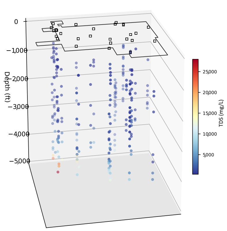
Compiling Existing Water-Quality Sample Data and Mapping It in 3D
Data are obtained from oil and water well records at each oil field.
Total Dissolved Solids (mg/L)
0
> 10,000
However, we do not have wells completed and water-sample data for much of the area where protected groundwater resources likely exist.
Using Geophysical Log Measurements Obtained When an Oil Well Is Drilled to Fill Gaps in Water-Quality Data
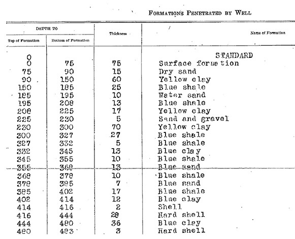
When oil wells are drilled, several different kinds of information may be collected, including information about the rocks and sediments and borehole geophysical logs. These geophysical logs measure various characteristics of the rocks and fluids and often include resistivity (or conductivity) data. Fluid salinity strongly affects resistivity values, and resistivity logs, in conjunction with porosity, self-potential, and gamma ray logs, can be used to calculate changes in salinity. Borehole geophysical log data from oil wells commonly span the depth intervals between where water and oil well casings are perforated and can be used to estimate salinity in these gaps.
Scanned images of borehole geophysical logs from most oil wells are available from the DOGGR; shown here are examples from different wells with scanned logs of lithology and geophysical sensor responses.
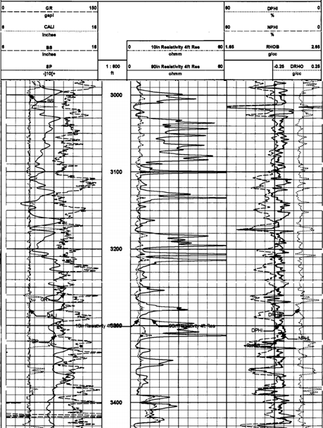
Using the Traced Geophysical Logs
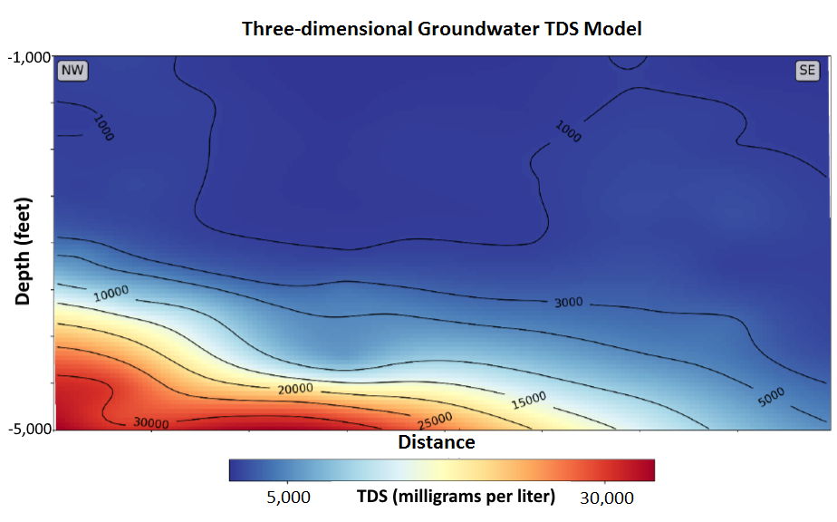
To calculate salinity along the depth profile of an individual well, we trace the resistivity lines on the scanned image to create a numerical record. We then calculate TDS values from selected intervals on the resistivity line that reflect the right conditions for applying salinity equations. Once we have calculated TDS points for multiple wells, we apply statistical techniques to generate a 3DTDS model across the landscape (Gillespie and others, 2017; Shimabukuro and Ducart, 2016; Shimabukuro and others, 2016; Stephens and others, 2018).
The basic procedure for digitizing scanned images is labor-intensive and finding more efficient techniques is important.
Using Ground-Based and Aerial EM Surveys to Map Subsurface
After compiling existing water-quality data and calculating salinity profiles from digitized oil well-log information, there are still gaps in groundwater salinity data between wells, especially in the buffer areas outside the oilfield footprint where there are fewer wells. Using EM techniques, subsurface resistivity can be surveyed from the surface or air, even for areas without wells (Fitterman and Stewart, 1986). The resulting resistivity model is somewhat similar to a low-resolution borehole resistivity log. By collecting these data near wells with logs, the interpretation of the EM data is grounded in independent data on lithology and salinity. We can then make interpretations about how the geologic structure and salinity change between wells are guided by the airborne and surface data collected between wells.
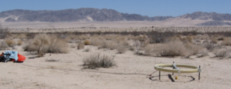
Ground-based EM system (Ball, L.B., written commun., 2017).
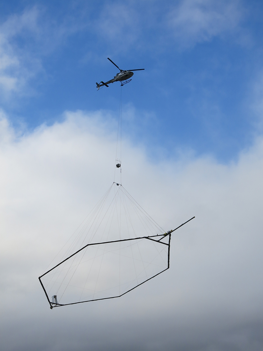
These EM surveys can be completed using geophysical instruments on the ground or suspended from aircraft. Ground measurements are useful to collect data in strategic locations at single sites, while airborne systems are able to efficiently collect high resolution data over large regions in a series of survey flight lines, usually arranged in blocks of evenly spaced lines.
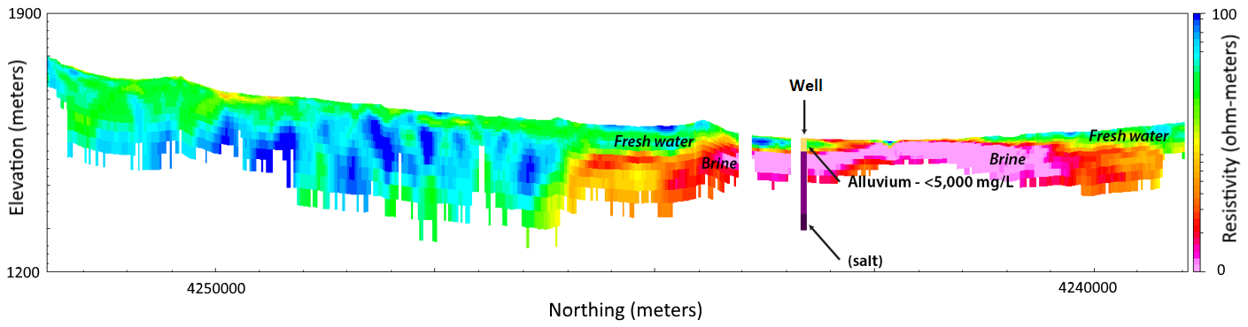
Airborne EM data can be used to create high-resolution cross sections and depth-slice maps of resistivity over large regions. These resistivity sections and maps can then be tied to salinity values from compiled water-quality data and digitized well-log information to map salinity changes between wells.
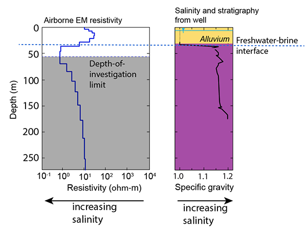
These two plots compare a resistivity model from an airborne EM survey of Paradox Valley, Colorado, to a measurement of salinity by depth at a nearby well (Ball and others, written commun., 2017). (Depth is in meters and resistivity is in Ohm-meters.)